Education / Selected work

The Central Limit Theorem, for two audiences

How much mathematics does a reader need to understand the same theorem?I wrote two versions of the central limit theorem around the same example: a four-page introduction requiring very little mathematical background, and a nine-page treatment proving the result through characteristic functions and Lévy’s continuity theorem. Both papers are in Dutch.

General reader Proof

One example, used twice

Both versions begin at the same coffee machine.

Suppose waiting times are exponentially distributed with rate λ = 1. The average wait is one minute, but individual waits are strongly skewed: most are short, while a few are much longer.

Now take groups of n people and record their average waiting time. For n = 1, nothing has changed: the distribution is still exponential. At n = 30, the picture is very different.

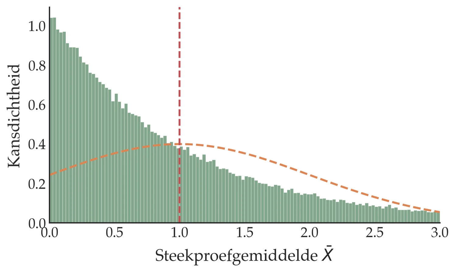
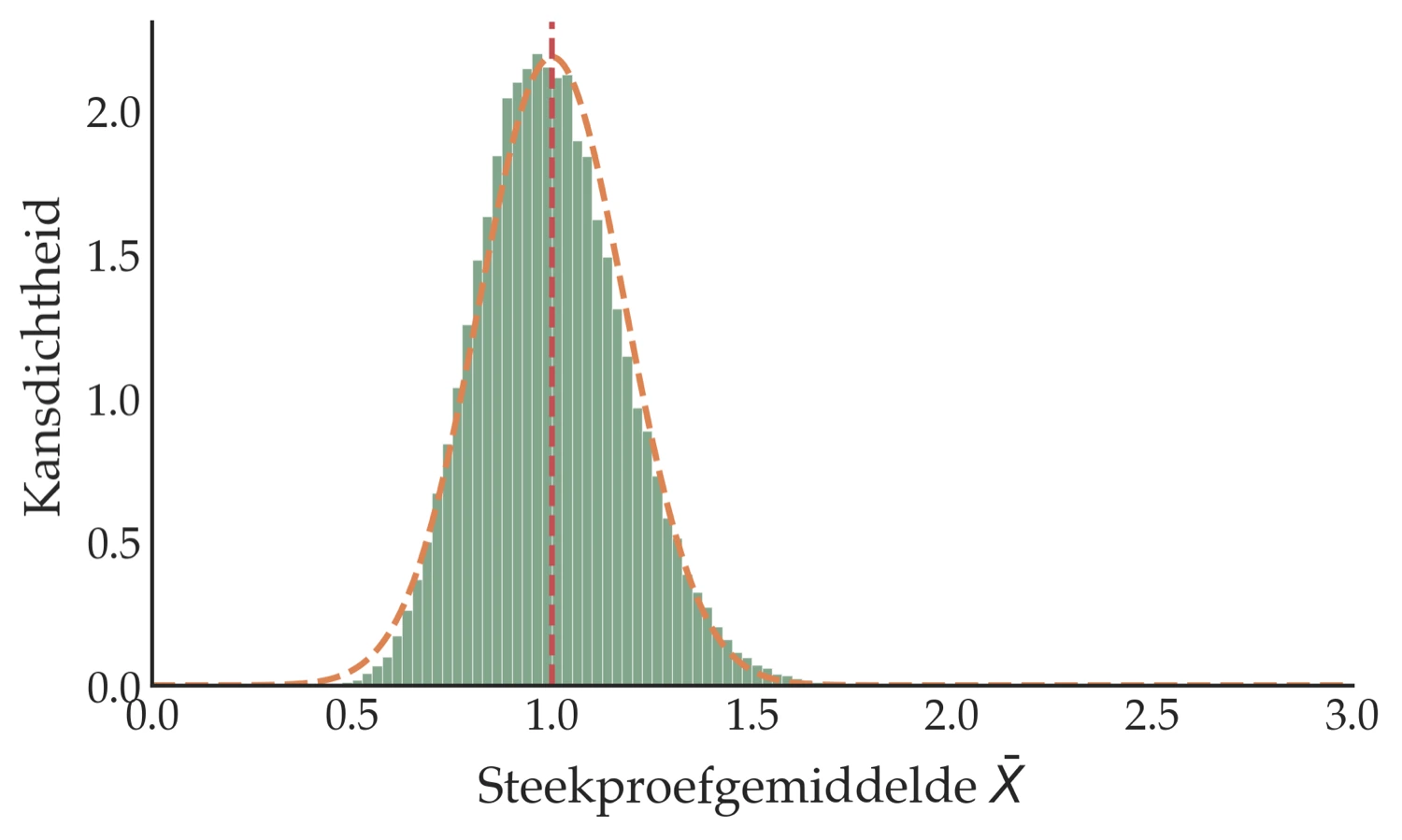
Histogram of 100,000 sample means at n = 1: a steeply falling, strongly right-skewed distribution, with a dashed normal curve that does not match it. — Distribution of the sample mean for n = 1, based on 100,000 simulations. The dashed curve is N(1, 1/n). Kansdichtheid is probability density; Steekproefgemiddelde X̄ is the sample mean.

Histogram of 100,000 sample means at n = 30: a narrow, near-symmetric bell closely tracked by the dashed normal curve. — The same experiment for n = 30. The distribution has narrowed and is already close to the corresponding normal curve.

The short paper stays with this experiment. The longer paper uses it as motivation before moving to the general theorem.

What the short version can show

For exponential observations, the distribution of the sample mean is known exactly:

\bar X_n \sim \Gamma\!\left(n,\tfrac{1}{n}\right)

That makes it possible to watch two things happen as n grows.

n	Spread 1/√n	Skewness 2/√n
1	1.000	2.000
2	0.707	1.414
5	0.447	0.894
30	0.183	0.365

Table 2 of the general-reader paper, reproduced to the digit it prints. The proof rounds the same skewness column to 2.00, 1.41, 0.89 and 0.37.

The averages become less dispersed, but they also become more symmetric. Both effects occur at a rate proportional to 1/√n.

That is enough to make the central limit theorem visible without asking the reader to accept a proof they cannot follow.

It also shows why the familiar rule that “n = 30is enough” should be treated as a rule of thumb rather than a theorem. At n = 30, the skewness is still 0.365: the distribution is close to normal, but it is not normal.

What the proof adds

The simulation shows what happens in one example. The longer paper asks the harder question: why should a normal distribution appear at all?

For independent and identically distributed variables with finite mean μ and variance σ², define

Y_i=\frac{X_i-\mu}{\sigma}, \qquad Z_n=\frac{1}{\sqrt{n}}\sum_{i=1}^{n} Y_i

The characteristic function of the sum becomes a product because the Yᵢ are independent:

\varphi_{Z_n}(t) = \left( \varphi_Y\!\left(\frac{t}{\sqrt{n}}\right) \right)^{n}

A second-order expansion around zero gives

\varphi_Y\!\left(\frac{t}{\sqrt{n}}\right) = 1-\frac{t^{2}}{2n}+o\!\left(\frac{1}{n}\right)

and therefore

\varphi_{Z_n}(t) = \left( 1-\frac{t^{2}}{2n}+o\!\left(\frac{1}{n}\right) \right)^{n} \longrightarrow e^{-t^{2}/2}

The limit e^(−t²/2)is the characteristic function of the standard normal distribution. Lévy’s continuity theorem then converts convergence of characteristic functions into convergence in distribution:

Z_n \xrightarrow{\;d\;} N(0,1)

That is the step the short version cannot provide: not merely that a bell curve appears in this example, but why it appears for a much larger class of distributions.

Where the assumptions matter

The finite-variance assumption is not decorative. It is what gives the characteristic function the second-order behaviour used in the proof.

A Cauchy distribution, for example, has neither a finite mean nor a finite variance. Averaging more Cauchy observations does not make the sample mean converge to a normal distribution; the central limit theorem simply does not apply.

That matters outside textbook examples. Heavy-tailed data, outliers and transformations cannot be treated as minor preprocessing details when they affect whether the assumptions behind the theorem are reasonable.

The two papers therefore end in slightly different places. The short version shows the phenomenon clearly enough to use it with care. The longer version explains why it works — and where it stops working.

General reader · 4 pp · NL Proof · 9 pp · NL

Written 15 June 2026. Both papers are in Dutch.

← Back to Education