Education | Selected work
Recovering the reproduction number from hospital admissions
Can the history of an epidemic be reconstructed from hospital admissions alone?I fitted a compartmental model to four years of Dutch COVID-19 hospital admissions and asked it to recover how transmission changed over time — without using case counts, test data or contact tracing. The recovered reproduction number was then compared with the series published independently by RIVM.
The question
The reproduction number is central to understanding an epidemic, but it is not observed directly. It has to be inferred from something we can count.
During COVID-19, positive tests were an obvious source. But testing behaviour changed continuously: capacity expanded, access changed, people became more or less willing to test, and many self-tests were never recorded.
Hospital admissions have a different character. They are not generated by a decision to seek a test, but by illness severe enough to require hospital care.
How much of the underlying transmission history can be recovered from hospital admissions alone?
Why use a compartmental model?
Hospital admissions tell us when people entered hospital. They do not directly tell us how many people were susceptible, infectious or recovered at that moment. Yet the reproduction number depends on precisely that hidden population state.
A SIRS model keeps track of it:
Rather than prescribing a fixed shape for transmission, β(t) is estimated from the admissions data itself. In the baseline model it is piecewise constant over 21-day intervals.
The model therefore has to infer both the hidden epidemic state and the transmission path that could have produced the observed hospitalisations.
Fitting four years of admissions
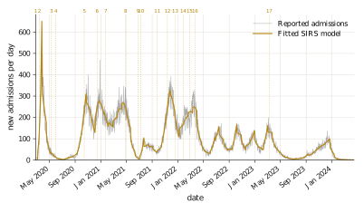
The model is fitted to 1,495 days of Dutch COVID-19 hospital admissions, from 27 February 2020 to 15 April 2024.
The baseline specification contains 75 free parameters: 72 transmission values, a hospitalisation ratio, an infection-to-admission delay and the initial infectious population. Parameters are estimated with bounded nonlinear least squares from 48 random starting points. The resulting fit reaches an RMSE of 25.1 hospital admissions per day.
The important test
A model reproducing the admissions curve does not necessarily mean it has recovered the transmission process that generated it. Fortunately, there is an independent comparison.
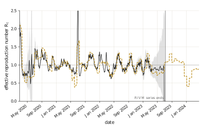
RIVM publishes its own estimate of the reproduction number, calculated using a different method and data stream. That series is never shown to the model during fitting. So after estimating the model, I compare its recovered Rt with RIVM’s published Rt.
At the model’s 21-day resolution:
- Correlation with RIVM
- 0.804
- Agreement on the direction of change
- 81.5%
- Intervals inside RIVM's 95% uncertainty band
- 50.0%
For comparison, the best constant reproduction number agrees on direction only 50% of the time and lies inside the RIVM interval in 38.9% of periods.
The surprising result
The model that fits hospital admissions best is not the model that recovers transmission best.
Reducing the transmission buckets gives the model more freedom. The admissions fit keeps improving:
- 84-day buckets
- RMSE 51.4
- 21-day buckets
- RMSE 25.1
- 7-day buckets
- RMSE 21.8
AIC therefore selects the most flexible 7-day model, with 219 parameters. But its correlation with RIVM falls to just 0.173 — the worst of every bucket width tested.
BIC instead selects the 21-day model. Its fit to admissions is slightly worse, but its recovered transmission history is substantially better.
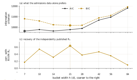
The interpretation is straightforward: beyond a certain point, additional parameters stop resolving genuine changes in transmission and start absorbing reporting noise. The model becomes better at reproducing what was observed while becoming worse at recovering what generated it.
A diagnostic without external data
Normally there is no independent Rt series available. If there were, there would be less reason to reconstruct it in the first place. That makes internal diagnostics important.
One useful parameter is the estimated delay between infection and hospital admission. We do not know its exact value, but we know approximately what is physiologically plausible.
At several over-flexible specifications, the estimated delay collapses to 1.8–2.2 days. At the 10- and 21-day resolutions it remains around 8.5–9.1 days. That gives a useful one-sided diagnostic:
An implausible delay is evidence against a model specification. A plausible delay does not, by itself, validate it.
Separating transmission from hospital delay
The model also separates two events that look almost identical in the raw admissions curve.
COVID measures took effect on 15 March 2020. Hospital admissions peaked 11 days later, on 26 March, measured on a centred seven-day mean. Taken literally, that could suggest that transmission continued rising for almost two weeks.
The fitted infection flux tells a different story. It peaks on 18 March — only three days after the measures. Most of the visible lag therefore comes afterwards, from the time between infection and hospital admission. The model independently estimates that delay at 9.1 days.
In other words, the hospital curve turned slowly because hospitals observe infections late.
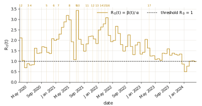
Across the full window, estimated R0(t) ranges from 0.50 to 3.43, with a mean of 1.72.
What verification caught
Three implementation errors materially changed the results despite leaving the fit looking reasonable.
- Missing observations were initially treated as zero admissions.
- The reporting delay was rounded to whole days, making its numerical gradient zero and preventing the optimiser from estimating it.
- The ODE solver stepped across discontinuities in β(t) without explicitly respecting the bucket boundaries.
None of these problems was obvious from goodness of fit alone. That became another lesson of the project: a convincing curve is not sufficient evidence that the model underneath it is behaving correctly.
Limits of the result
This is a retrospective reconstruction, not a real-time estimator. The model sees the full four-year window at once, so early estimates benefit from later data.
The hospitalisation ratio is also held constant despite vaccination, variants and changing population immunity. That is a strong simplification and likely affects the absolute scale of R0(t), particularly after 2021.
The model is therefore stronger at recovering the shape and timing of transmission than its absolute magnitude. And any counterfactual produced by the model should be read as a statement about the fitted system, not a direct claim about what would have happened in the Netherlands.
Written for Simuleren en Modelleren · BSc Mathematics · University of Amsterdam · January 2026. Revised and published September 2026.